slam
A Continuous-time VINS
S. Lovegrove, A. Patron-Perez, and G. Sibley, “Spline Fusion: A continuous-time representation for visual-inertial fusion with application to rolling shutter cameras,” in Procedings of the British Machine Vision Conference 2013, Bristol: British Machine Vision Association, 2013, p. 93.1-93.11. doi: 10.5244/C.27.93.
这篇论文主要工作是建立了卷帘相机的连续时域下的数学模型,初始化方法是利用 IMU 主动对齐视觉。
相比离散时域,在连续时域上表示有助于融合高帧率的传感器和异步时间戳的设备。对卷帘相机的研究尚未成熟,现有的工作主要集中在如何消除卷帘相机的畸变,而后复用标准全局快门相机的 SLAM 模型,这种解耦合的处理方式增加了无法修正的偏差。
单目视觉系统存在 7 自由度不可观:6 自由度姿态+尺度,一种方法通过回环检测和序列图松弛对尺度显式参数化,另一种方法是加入可以测量绝对尺度的设备。在本文中作者使用了惯性单元。相比过往建立在欧拉角上的数学表示,作者引入李群和李代数上的旋转表示避免了奇异点,同时能够更好地近似最小扭矩的轨迹。
\[
\mathbf T_{b,a} = \begin{bmatrix}
\mathbf R_{b,a} & \mathbf a_b \\
\mathbf 0^T & 1
\end{bmatrix},\ \mathbf T_{b,a}\in\mathbb{SE}3,\ \mathbf R_{b,a}\in\mathbb{SO}3
\]
作者希望轨迹的参数化方程是局部可控,二阶导连续,能近似最小力矩轨迹的。三次 B 样条曲线可以很好表示 \(\mathbb R^3\) 上的轨迹,但在三维旋转上表现一般。因此作者选用了李代数上的累计基函数,这种函数最早被应用在计算机动画中的四元数插值中。
自由度为 \(k-1\) 的 B 样条曲线的标准基函数表示为
\[
\begin{aligned}
\mathbf p(t) &= \sum_{i=0}^n\mathbf p_i B_{i,k}(t) \\
&= \mathbf p_0 B_{0,k}(t) + \mathbf p_1 B_{1,k}(t) + \cdots + \mathbf p_n B_{n,k}(t) \\
&= \mathbf p_0B_{0,k}(t) + \sum_{i=1}^{n-1}\mathbf p_iB_{i,k}(t) + \mathbf p_nB_{n,k}(t) \\
&= \mathbf p_0\tilde B_{0,k}(t) + \sum_{i=1}^n\mathbf p_i\sum_{j=i}^nB_{j,k}(t) - \sum_{i=0}^{n-1}\mathbf p_i\sum_{j=i+1}^nB_{j,k}(t) \\
&= \mathbf p_0\tilde B_{0,k}(t) + \sum_{i=1}^n(\mathbf p_i-\mathbf p_{i-1})\tilde B_{i,k}(t)
\end{aligned}
\]
其中 \(\mathbf p_i\in\mathbb R^N\) 是在 \(t_i,i\in[0,\dots,n]\) 时刻的控制点,\(B_{i,k}(t)\) 是由德伯尔-考克斯递归公式 De Boor - Cox recursive formula 计算得到的基函数。进一步利用李群的指数映射和对数映射,将公式重写在李群域上
\[
\mathbf T_{w,s}(t) = \exp(\tilde B_{0,k}\log(\mathbf T_{w,0}))\prod_{i=1}\exp(\tilde B_{i,k}(t)\log(\mathbf T_{w,i-1}^{-1}\mathbf T_{w,i}))
\]
作者进一步在假设控制点时间间隔不变的情况下(大多数单目系统应该都能满足),对时间做了归一化处理
\[
u(t) = \frac{t-t_0}{\Delta t} - s_i
\]
并在参数 \(k=4\) 下转化为矩阵表达
\[
\tilde{\mathbf B}(u) = \mathbf C\begin{bmatrix}1\\u\\u^2\\u^3\end{bmatrix},\dot{\tilde{\mathbf B}}(u) = \mathbf C\begin{bmatrix}0\\1\\2u\\3u^2\end{bmatrix},\ddot{\tilde{\mathbf B}}(u) = \mathbf C\begin{bmatrix}0\\0\\2\\6u\end{bmatrix},\mathbf C=\frac16\begin{bmatrix}6&0&0&0\\5&3&-3&1\\1&3&3&-2\\0&0&0&1\end{bmatrix}
\]
\[
\mathbf T_{w,s}(u) = \mathbf T_{w,i-1}\prod_{j=1}^3\exp(\tilde{\mathbf B}(u)_j\log(\mathbf T_{w,i+j-1}^{-1}\mathbf T_{w,i+j}))
\]
\(\dot{\mathbf T}_{w,s},\ddot{\mathbf T}_{w,s}\) 则由链式法则和指数映射的一阶近似得到
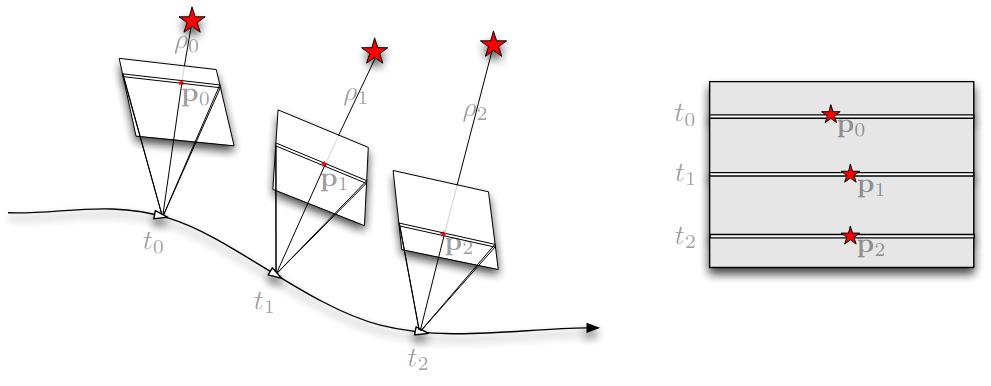
给定第一次观测的逆深度 \(\mathbb Rho\in\mathbb R^+\) , 对应点在两帧的坐标分别为 \(\mathbf p_a,\mathbf p_b\in\mathbb R^2\) , 其中 \(\pi(\mathbf P)=\frac1{P_2}[P_0,P_1]^T\)
\[
\mathbf p_b = \mathcal W(\mathbf p_a;\mathbf T_{b,a},\mathbb Rho)=\pi\bigg(\begin{bmatrix}\mathbf K_b&\mathbf 0\end{bmatrix}\mathbf T_{b,a}\begin{bmatrix}\mathbf K_a^{-1}\begin{bmatrix}\mathbf p_a\\1\end{bmatrix}&\mathbb Rho\end{bmatrix}\bigg)
\]
对于一般的视觉惯性系统给出损失函数
\[
\begin{aligned}
E(\theta) =& \sum_{\hat{\mathbf p}_m}\left[\hat{\mathbf p}_m-\mathcal W(\mathbf p_r;\mathbf T_{c,s}\mathbf T_{w,s}(u_m)^{-1}\mathbf T_{w,s}(u_r)\mathbf T_{s,c},\rho)\right]_{\Sigma_p}^2 +\\
& \sum_{\hat\omega_m}[\hat\omega_m-\text{Gyro}(u_m)]_{\Sigma_\omega}^2 + \sum_{\hat{\mathbf a}_m}[\hat{\mathbf a}_m-\text{Accel}(u_m)]^2_{\Sigma_\mathbf a}
\end{aligned}
\]
而对卷帘相机则将 \(\mathbf p_b\) 用 \(\mathbf p_b(t)\) 替代重新建模
\[
\mathbf p_b(t) = \begin{bmatrix}
x_b(t) \\ y_b(t)
\end{bmatrix} = \mathcal W(\mathbf p_a;\mathbf T_{b,a}(t),\rho)
\]
\[
\mathbf p_b(t+\Delta t) = \mathcal W(\mathbf p_a;\mathbf T_{b,a}(t),\rho) + \Delta t\cdot\frac{\partial}{\partial t}\mathcal W(\mathbf p_a;\mathbf T_{b,a}(t),\rho)
\]
\[
y_b(t+\Delta t) = \frac{h(t+\Delta t-s)}{e-s},\quad\Delta t=-\frac{h\cdot t_0+s\cdot(y_b(t)-h)-e\cdot y_b(t)}{(s-e)\frac{\partial}{\partial t}\mathcal W_y(\mathbf p_a;\mathbf T_{b,a}(t),\rho)+h}
\]
这一系统表现出了良好的自校准的能力