math
slam
M. R. Walter, R. M. Eustice, and J. J. Leonard, “Exactly Sparse Extended Information Filters for Feature-based SLAM,” The International Journal of Robotics Research , vol. 26, no. 4, pp. 335–359, Apr. 2007, doi: 10.1177/0278364906075026 .
稀疏扩展信息滤波器(SEIF)SLAM 是一种计算高效的同时定位与地图构建(SLAM)方法。通过利用信息矩阵的稀疏性,SEIF 降低了状态估计的计算复杂度,使其适用于大规模环境。
Gaussian Probability
对服从高斯分布的多元随机变量 \(\mathbf\xi_t\sim\mathcal N(\boldsymbol\mu_t,\Sigma_t)\) 可以通过均值向量 \(\boldsymbol\mu_t\) 和协方差矩阵 \(\Sigma_t\) 参数化,同时也可以被规范形式 \(\mathcal N^{-1}(\boldsymbol\eta_t,\Lambda_t)\) 所表示,其中 \(\Lambda_t=\Sigma_t^{-1},\boldsymbol\eta_t=\Sigma^{-1}_t\boldsymbol\mu_t\) .
\[
\begin{aligned}
p(\xi_t) &= N(\mu_t, \Sigma_t) \\
&\propto \exp\left\{-\frac{1}{2}(\xi_t - \mu_t)^\top \Sigma_t^{-1}(\xi_t - \mu_t)\right\} \\
&= \exp\left\{-\frac{1}{2}(\xi_t^\top \Sigma_t^{-1} \xi_t - 2\mu_t^\top \Sigma_t^{-1} \xi_t + \mu_t^\top \Sigma_t^{-1} \mu_t)\right\} \\
&\propto \exp\left\{-\frac{1}{2}\xi_t^\top \Sigma_t^{-1} \xi_t + \mu_t^\top \Sigma_t^{-1} \xi_t\right\} \\
&= \exp\left\{-\frac{1}{2}\xi_t^\top \Lambda_t \xi_t + \eta_t^\top \xi_t\right\} \propto N^{-1}(\eta_t, \Lambda_t)
\end{aligned}
\]
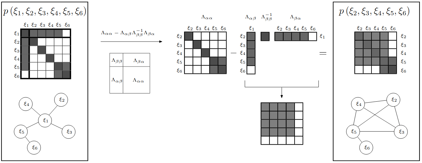
在标准形式中,边缘化操作只需从均值向量和协方差矩阵中移除相应的元素。然而在规范形式中,边缘化操作需要计算舒尔补 ,计算复杂度较高。条件化则相反,在标准形式中操作较为复杂,在规范形式下则相对简单。
Implied Conditional Independence
\[
\begin{aligned}
p(\boldsymbol\xi)&\propto\exp\left\{-\frac12\boldsymbol\xi^T\Lambda\boldsymbol\xi+\boldsymbol\eta^T\boldsymbol\xi\right\} \\
&= \exp\left\{\sum_i\left(\eta_i\xi_i-\frac12\sum_j\xi_i\lambda_{ij}\xi_j\right)\right\} \\
&=\prod_i\exp\left\{-\frac12\lambda_{ii}\xi_i^2+\eta_i\xi_i\right\}\cdot\prod_{i\neq j}\exp\left\{-\frac12\xi_i\lambda_{ij}\xi_j\right\} \\
&= \prod_i\Psi_i(\xi_i)\cdot\prod_{i\ne j}\Psi_{ij}(\xi_i,\xi_j)
\end{aligned}
\]
其中
\[
\begin{aligned}
\Psi_i(\xi_i) &= \exp\left\{-\frac12\lambda_{ii}\xi_i^2+\eta_i\xi_i\right\} \\
\Psi_{ij}(\xi_i,\xi_j) &= \exp\left\{-\frac12\xi_i\lambda_{ij}\xi_j\right\}
\end{aligned}
\]
“The meaning of a zero in an inverse covariance matrix (at location \(i, j\) ) is conditional on all the other variables, these two variables \(i\) and \(j\) are independent. ... So positive off-diagonal terms in the covariance matrix always describe positive correlation; but the off-diagonal terms in the inverse covariance matrix can’t be interpreted that way. The sign of an element \((i, j)\) in the inverse covariance matrix does not tell you about the correlation between those two variables.” (MacKay and Cb, 2006, p. 4)
如果信息矩阵中的非对角元素为零,即 \(\lambda_{ij} = 0 \Leftrightarrow \Psi_{ij}(\xi_i, \xi_j) = 1\) ,这意味着两个节点之间没有边约束,表明 \(\xi_i\) 和 \(\xi_j\) 条件独立。相反,如果非对角元素不为零,则表明 \(\xi_i\) 和 \(\xi_j\) 之间存在一条边约束,其强度正比于 \(\lambda_{ij}\) 。这种关系很好地体现在无向图中,直观地反映了变量之间的条件独立性。使用规范形式的一个主要好处是,信息矩阵 \(\Lambda\) 提供了马尔可夫场的显式结构表示,清晰地揭示了变量之间的依赖关系。关于协方差矩阵和信息矩阵的更多深入理解,可以参考 David J.C. MacKay 2006 年的手稿 The Humble Gaussian Distribution .
\[
p(\boldsymbol\xi_t|\mathbf z^t,\mathbf u^t)=\mathcal N(\boldsymbol\mu_t,\Sigma_t)=\mathcal N^{-1}(\boldsymbol\eta_t,\Lambda_t)
\]
记状态 \(\boldsymbol\xi_t=[\mathbf x_t^T\quad\mathbf M_t^T]^T\) 为机器人位姿为 \(\mathbf x_t\) 和地图特征 \(\mathbf M=\set{\mathbf m_1,\cdots,\mathbf m_n}\) 的组合,\(\mathbf z^{1:t}\) 和 \(\mathbf u^{1:t}\) 表示观测数据和输入的历史。地图基于信息矩阵的结构被划分为两个集合,\(\mathbf M = (\mathbf m^+,\mathbf m^-)\) ,其中 \(\mathbf m^+\) 包含那些与机器人存在非零非对角项连接的地图元素,而 \(\mathbf m^-\) 则表示与车辆位姿条件独立的特征。
Measurement Update Step
观测对减小机器位姿和地图的估计的不确定性有重要影响,在均值处对非线性观测模型做一阶近似
\[
\begin{aligned}
\mathbf z_t &= \mathbf h(\boldsymbol\xi_t)+\mathbf v_t \\
&\approx\mathbf h(\bar{\boldsymbol\mu}_t)+H(\boldsymbol\xi_t-\bar{\boldsymbol\mu}_t)+\mathbf v_t,\quad\mathbf v_t\sim\mathcal N(0,R)
\end{aligned}
\]
根据马尔科夫假设 \(p(\mathbf z_t|\boldsymbol\xi_t,\mathbf z_{1:t-1},\mathbf u_{1:t})=p(\mathbf z_t|\boldsymbol\xi_t)\) 和 \(\forall\boldsymbol\xi_t,p(\mathbf z_t|\mathbf z_{1:t-1}\mathbf u_{1:t})=\frac1\eta\) ,贝叶斯定理给出
\[
\begin{aligned}
p(\boldsymbol\xi_t|\mathbf z_{1:t},\mathbf u_{1:t}) &= p(\boldsymbol\xi_t|\mathbf z_t,\mathbf z_{1:t-1},\mathbf u_{1:t}) \\
&= \frac{p(\mathbf z_t|\boldsymbol\xi_t,\mathbf z_{1:t-1},\mathbf u_{1:t})\cdot p(\boldsymbol\xi_t|\mathbf z_{1:t-1},\mathbf u_{1:t})}{p(\mathbf z_t|\mathbf z_{1:t-1},\mathbf u_{1:t})} \\
&= \eta\cdot p(\mathbf z_t|\boldsymbol\xi_t)\cdot p(\boldsymbol\xi_t|\mathbf z_{1:t-1},\mathbf u_{1:t})\\
&= \mathcal N^{-1}(\boldsymbol\eta_t,\Lambda_t)
\end{aligned}
\]
在更新时,EIF 估计规范形式的新的后验概率
\[
\begin{aligned}
\Lambda_t &= \bar\Lambda_t+H^TR^{-1}H \\
\boldsymbol\eta_t &= \bar{\boldsymbol\eta}_t + H^TR^{-1}(\mathbf z_t-\mathbf h(\bar{\boldsymbol\mu}_t)+H\bar{\boldsymbol\mu}_t)
\end{aligned}
\]
其中测量模型是一个只包含机器当前位姿以及现在观测到的地标的函数,在雅可比中表现为极度稀疏(没观测到的地标的梯度为 \(0\) )
\[
H=\begin{bmatrix}
\frac{\partial h_1}{\partial\boldsymbol\xi_t} & \cdots & \mathbf 0 & \cdots & \frac{\partial h_1}{\partial\mathbf m_i} & \cdots & \mathbf 0 \\
\vdots & & & \ddots & & & \vdots \\
\frac{\partial h_m}{\partial\boldsymbol\xi_t} & \cdots & \frac{\partial h_m}{\partial\mathbf m_j} & \cdots & \mathbf 0 & \cdots & \mathbf 0 \\
\end{bmatrix}
\]
信息矩阵通过稀疏矩阵 \(H^TR^{-1}H\) 进行更新,仅修改与机器人位姿和观测地标相关的项,从而加强或建立新的约束;由于 \(H\) 的稀疏性和机器人视野的限制,更新时间与观测数量 \(m\) 相关,复杂度为 \(\mathcal O(m^2)\) ,且不随地图规模增长;在非线性情况下,计算均值需要 \(\mathcal O(n^3)\) 的矩阵求逆,而在线性情况下,更新可以在常数时间内完成,无需均值计算。
Time Projection Step
时间预测包括状态扩展和边缘化。首先参考观测模型,对于运动学模型我们同样给出一阶近似
\[
\begin{aligned}
\mathbf x_{t+1} &= \mathbf f(\mathbf x_t,\mathbf u_{t+1})+\mathbf w_t \\
&\approx \mathbf f(\boldsymbol\mu_{\mathbf x_t},\mathbf u_{t+1}) + F(\mathbf x_t - \boldsymbol\mu_{\mathbf x_t}) + \mathbf w_t,\quad\mathbf w_t\sim\mathcal N(0,Q)
\end{aligned}
\]
首先将新的机器人位姿加入状态向量,并同步扩展信息矩阵和信息向量。其中状态向量 \(\hat{\boldsymbol\xi}_{t+1}=[\mathbf x_t^T,\mathbf x_{t+1}^T,\mathbf M^T]^T\) 遵循后验分布 \(p(\boldsymbol\xi_t|\mathbf z_{1:t},\mathbf u_{1:t}) = \mathcal N^{-1}(\boldsymbol\eta_t,\Lambda_t)\) . 如图所示,根据马尔科夫性质,新的位姿只和上一步位姿相关而与地图无关。
\[
\begin{aligned}
p(\hat{\boldsymbol\xi}_{t+1}|\mathbf z_{1:t},\mathbf u_{1:t+1}) &= p(\mathbf x_{t+1},\boldsymbol\xi_t|\mathbf z_{1:t},\mathbf u_{1:t+1}) \\
&= p(\mathbf x_{t+1}|\mathbf x_t,\mathbf u_{t+1})\cdot p(\boldsymbol\xi_t|\mathbf z_{1:t},\mathbf u_{1:t})
\end{aligned}
\]
新的状态估计服从更新后的高斯分布
\[
p(\mathbf x_t,\mathbf x_{t+1},\mathbf M|\mathbf z_{1:t},\mathbf u_{1:t+1})=\mathcal N(\hat{\boldsymbol\mu}_{t+1},\hat\Sigma_{t+1})=\mathcal N^{-1}(\hat{\boldsymbol\eta}_{t+1},\hat\Lambda_{t+1})
\]
\[
\begin{aligned}
\hat\Sigma_{t+1} &= \left[\begin{array} {c | c c}
\Sigma_{\mathbf x_t\mathbf x_t} & \rm F\Sigma_{\mathbf x_t\mathbf x_t} & \rm F\Sigma_{\mathbf x_t\mathbf M} \\
\hline
\rm\Sigma_{\mathbf x_t\mathbf x_t}F^T & \rm F\Sigma_{\mathbf x_t\mathbf x_t}F^T+Q & \Sigma_{\mathbf x_t\mathbf M} \\
\rm\Sigma_{\mathbf M\mathbf x_t}F^T & \Sigma_{\mathbf M\mathbf x_t} & \Sigma_{\mathbf M\mathbf M}
\end{array}\right]=\left[\begin{array} {c | c}
\hat\Sigma_{t+1}^{11} & \hat\Sigma_{t+1}^{12} \\
\hline
\hat\Sigma_{t+1}^{21} & \hat\Sigma_{t+1}^{22}
\end{array}\right]\\
\hat{\boldsymbol\mu}_{t+1} &= \left[\begin{array} c
\boldsymbol\mu_{\mathbf x_t} \\
\hline
\mathbf f(\boldsymbol\mu_{\mathbf x_t,\mathbf u_{t+1}}) \\
\boldsymbol\mu_{\mathbf M}
\end{array}\right]=\left[\begin{array} c
\hat{\boldsymbol\mu}_{t+1}^1\\\hline\hat{\boldsymbol\mu}_{t+1}^2
\end{array}\right]
\end{aligned}
\]
由协方差矩阵和信息矩阵的对偶性得到
\[
\begin{aligned}
\hat\Lambda_{t+1} &= \left[\begin{array} {c | c c}
\Lambda_{\mathbf x_t\mathbf x_t}+\rm FQ^{-1}F & \rm-F^TQ^{-1} & \Lambda_{\mathbf x_t\mathbf M} \\
\hline
\rm-Q^{-1}F & \rm Q^{-1} & 0 \\
\Lambda_{\mathbf M\mathbf x_t} & 0 & \Lambda_{\mathbf M\mathbf M}
\end{array}\right] = \left[\begin{array} {c | c}
\hat\Lambda_{t+1}^{11} & \hat\Lambda_{t+1}^{12} \\
\hline
\hat\Lambda_{t+1}^{21} & \hat\Lambda_{t+1}^{22}
\end{array}\right]\\
\hat{\boldsymbol\eta}_{t+1} &= \left[\begin{array} c
\boldsymbol\eta_{\mathbf x_t}-\rm F^TQ^{-1}[\mathbf f(\boldsymbol\mu_{\mathbf x_t,\mathbf u_{t+1}})-F\boldsymbol\mu_{\mathbf x_t}] \\
\hline
\rm Q^{-1}[\mathbf f(\boldsymbol\mu_{\mathbf x_t,\mathbf u_{t+1}})-F\boldsymbol\mu_{\mathbf x_t}] \\
\boldsymbol\eta_{\mathbf M}
\end{array}\right]=\left[\begin{array} c
\hat{\boldsymbol\eta}_{t+1}^1\\\hline\hat{\boldsymbol\eta}_{t+1}^2
\end{array}\right]
\end{aligned}
\]
第二步是边缘化 \(\mathbf x_t\) , 使状态向量变为 \(\boldsymbol\xi_{t+1}=[\mathbf x_{t+1}^T,\mathbf M^T]^T\) .
\[
\begin{aligned}
p(\mathbf x_{t+1},\mathbf M|\mathbf z_{1:t},\mathbf u_{1:t+1}) &= \int_{\mathbf x_t}p(\mathbf x_t,\mathbf x_{t+1},\mathbf M|\mathbf z_{1:t},\mathbf u_{1:t+1}){\rm d}\mathbf x_t \\
p(\boldsymbol\xi_{t+1}|\mathbf z_{1:t},\mathbf u_{1:t+1}) &=\mathcal N^{-1}(\bar{\boldsymbol\eta}_{t+1},\bar\Lambda_{t+1})
\end{aligned}
\]
\(\bar{\boldsymbol\eta}_{t+1}\) 和 \(\bar\Lambda_{t+1}\) 由前面表中给出的边缘化公式得到
\[
\begin{aligned}
\bar\Lambda_{t+1} &= \hat\Lambda_{t+1}^{22} - \hat\Lambda_{t+1}^{21}(\hat\Lambda_{t+1}^{11})^{-1}\hat\Lambda_{t+1}^{12} \\
\bar{\boldsymbol\eta}_{t+1} &= \hat{\boldsymbol\eta}_{t+1}^2 - \hat\Lambda_{t+1}^{21}(\hat\Lambda_{t+1}^{11})^{-1}\hat{\boldsymbol\eta}_{t+1}^1
\end{aligned}
\]
虽然 EIF 能高效处理新观测的增量更新,但通过边缘化旧位姿时产生的全连接问题会导致信息矩阵迅速稠密化,使得运动预测的计算复杂度达到 \(\mathcal O(n^2)\) 量级。边缘化过程会在新位姿与被移除旧位姿关联的所有特征 \(\mathbf m^+\) 之间建立新的信息连接,导致信息矩阵稠密化。但由于这些新连接通常具有较弱的关联强度,这为通过稀疏化近似来维持计算效率提供了可能,即保留强连接舍弃弱连接。
Active Sparsity Maintenance
记原先激活后续变为被动的特征为 \(\mathbf m^0\) ,则地图被划分为 \(\mathbf M=\set{\mathbf m^0,\mathbf m^+,\mathbf m^-}\) 三部分。下图表明通过主动控制激活特征断开,可以有效控制信息矩阵的稀疏性。而对与机器无关联的地标 \(\mathcal m^-\) ,我们可以任意给出估计 \(\boldsymbol\phi\) ,但实际上如果用了非均值的估计会使 SEIF 失准。
SEIF 给出去除 \(\mathbf m^0\) 后的近似后验估计
\[
\begin{aligned}
\tilde p_\text{SEIF}(\boldsymbol\xi_t|\mathbf z_{1:t},\mathbf u_{1:t}) &= \tilde p_\text{SEIF}(\mathbf x_t,\mathbf m^0,\mathbf m^+,\mathbf m^-|\mathbf z_{1:t},\mathbf u_{1:t}) \\
&= p(\mathbf x_t|\mathbf m^+,\mathbf m^-=\boldsymbol\phi,\mathbf z_{1:t},\mathbf u_{1:t})\cdot p(\mathbf m^0,\mathbf m^+,\mathbf m^-,\mathbf z_{1:t},\mathbf u_{1:t})
\end{aligned}
\]
Discussion on Overconfidence
假设三元变量 \([a,b,c]\) 服从高斯分布
\[
\begin{aligned}
p(a,b,c) &= \mathcal N\left(\begin{bmatrix}\mu_a\\\mu_b\\\mu_c\end{bmatrix},\begin{bmatrix}\sigma_a^2&\rho_{ab}\sigma_a\sigma_b&\rho_{ac}\sigma_a\sigma_c\\\rho_{ab}\sigma_a\sigma_b&\sigma_b^2&\rho_{bc}\sigma_b\sigma_c\\\rho_{ac}\sigma_a\sigma_c&\rho_{bc}\rho_b\rho_c&\sigma_c^2\end{bmatrix}\right) \\
&= \mathcal N^{-1}\left(\begin{bmatrix}\eta_a\\\eta_b\\\eta_c\end{bmatrix},\begin{bmatrix}\lambda_{aa}&\lambda_{ab}&\lambda_{ac}\\\lambda_{ab}&\lambda_{bb}&\lambda_{bc}\\\lambda_{ac}&\lambda_{bc}&\lambda_{cc}\end{bmatrix}\right)
\end{aligned}
\]
并且变量 \(a,b\) 在条件 \(c\) 下独立,将近似结果记为 \(\tilde p(a,b,c)\)
\[
p(a,b,c)=p(a,b|c)\cdot p(c)\approx p(a|c)\cdot p(b|c)\cdot p(c)=\tilde p(a,b,c)
\]
对于在 \(c\) 条件下条件独立的 \(a\) 和 \(b\) , 前面讨论过合适的做法是把信息矩阵的 \(\lambda_{ab}\) 设为 \(0\) , 这等价于协方差矩阵变为
\[
\tilde p(a,b,c) = \mathcal N\left(\begin{bmatrix}\mu_a\\\mu_b\\\mu_c\end{bmatrix},\begin{bmatrix}\sigma_a^2&\rho_{ac}\rho_{bc}\sigma_a\sigma_b&\rho_{ac}\sigma_a\sigma_c\\\rho_{ac}\rho_{bc}\sigma_a\sigma_b&\sigma_b^2&\rho_{bc}\sigma_b\sigma_c\\\rho_{ac}\sigma_a\sigma_c&\rho_{bc}\rho_b\rho_c&\sigma_c^2\end{bmatrix}\right) \\
\]
为了保证近似后的一致性,一个充要条件是 \(\bar\Sigma-\Sigma\) 半正定
\[
\bar\Sigma-\Sigma=\begin{bmatrix}
0 & (\rho_{ac}\rho_{bc}-\rho_{ab})\sigma_a\sigma_b & 0 \\
(\rho_{ac}\rho_{bc}-\rho_{ab})\sigma_a\sigma_b & 0 & 0 \\
0 & 0 & 0
\end{bmatrix}\succeq0
\]
其中,一个使 \(\bar\Sigma-\Sigma\) 半正定的必要条件是左上的 \(2\times2\) 子矩阵非负。
\[
\text{det}\left(\begin{bmatrix}
0 & (\rho_{ac}\rho_{bc}-\rho_{ab})\sigma_a\sigma_b \\
(\rho_{ac}\rho_{bc}-\rho_{ab})\sigma_a\sigma_b & 0 \\
\end{bmatrix}\right)=-[(\rho_{ac}\rho_{bc}-\rho_{ac})\sigma_a\sigma_b]^2\le0
\]
只有在 \(\rho_{ab}=\rho_{ac}\rho_{bc}\) 时 \(\bar\Sigma-\Sigma\) 半正定,否则强制稀疏化会导致信息矩阵过于自信,即信息矩阵被过度强化,导致估计的协方差比实际小。