math
slam
Derivation of On-Manifold IMU Preintegration
C. Forster, L. Carlone, F. Dellaert, and D. Scaramuzza, “On-Manifold Preintegration for Real-Time Visual--Inertial Odometry,” IEEE Trans. Robot. , vol. 33, no. 1, pp. 1–21, Feb. 2017, doi: 10.1109/TRO.2016.2597321 .
Z. Yang and S. Shen, “Monocular Visual–Inertial State Estimation With Online Initialization and Camera–IMU Extrinsic Calibration,” IEEE Trans. Automat. Sci. Eng., vol. 14, no. 1, pp. 39–51, Jan. 2017, doi: 10.1109/TASE.2016.2550621.
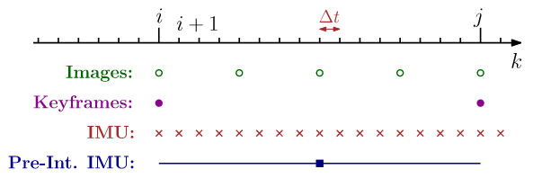
IMU preintegration is a technique in visual-inertial odometry that efficiently fuses high-frequency IMU data between keyframes. Using Lie group theory on \(SE(3)\) , it handles nonlinear 3D rotations and precomputes motion constraints for optimization. This method accounts for sensor biases, noise, and is essential for real-time state estimation.
Special Orthology Group \(SO(3)\)
The special orthology group \(SO(3)\) is defined as the set of all \(\mathbb{R}^{3\times3}\) rotation matrix:
\[
SO(3) = \set{R\in\mathbb{R}^{3\times3}:R^TR=I,\det(R)=1}
\]
And its tagent space on the manifold \(\mathfrak {so}(3)\) , consist of skew-symmetric matrices:
\[
\boldsymbol\omega^\wedge = \begin{bmatrix}
\omega_1 \\ \omega_2 \\ \omega_3
\end{bmatrix}^\wedge = \begin{bmatrix}
0 & -\omega_3 & \omega_2 \\
\omega_3 & 0 & -\omega_1 \\
-\omega_2 & \omega_1 & 0 \\
\end{bmatrix} \in \mathfrak{so}(3) \tag{1}
\]
The hat operator \((\cdot)^\wedge\) maps a vector \(\boldsymbol\omega\in\mathbb{R}^3\) to \(\mathfrak{so}(3)\) , while the vee operator \((\cdot)^\vee\) performs the inverse mapping.
Rodrigues' Rotation Formula
Let \(\bf v\in\mathbb{R}^3\) be a 3D vector to be rotated by a unit vector axis \(\bf n=\begin{pmatrix}n_x\\n_y\\n_z\end{pmatrix}\) by an angle \(\theta\) . The resulting rotated vector is denoted \(\bf v_\text{rot}\) .
\(\bf v\) can be decomposed to two orthogonal components: the parallel to \(\bf n\) part \(\bf v_\parallel\) and the perpendicular to \(\bf n\) part \(\bf v_\perp\) . Which satisfy,
\[
\begin{cases}
\mathbf v_\parallel = (\mathbf v\cdot\mathbf n)\mathbf n \\
\mathbf v_\perp = \mathbf v-(\mathbf v\cdot\mathbf n)\mathbf n = -\mathbf n\times(\mathbf n\times\mathbf v)
\end{cases}
\]
The whole vector \(\bf v\) is then rotated by:
\[
\begin{aligned}
\mathbf v_\text{rot} &= \mathbf v_{\parallel \text{rot}} + \mathbf v_{\perp \text{rot}} \\
&= \mathbf v_\parallel + \cos\theta\mathbf v_\perp + \sin\theta\mathbf n\times\bf v_\perp \\
&= (\mathbf v\cdot\mathbf n)n + \cos\theta\mathbf v_\perp + \sin\theta\mathbf n\times\mathbf v \\
&= \cos\theta\mathbf v+(1-\cos\theta)(\mathbf n\cdot\mathbf v)\mathbf n + \sin\theta\mathbf n\times\mathbf v
\end{aligned}
\]
We get Rodrigues' Rotation Formula. Write it on the manifold, we then have:
\[
R = \cos(||\phi||)I+[1-\cos(||\phi||)]\frac{\phi\phi^T}{||\phi||^2} + \sin(||\phi||)\phi^\wedge
\]
The exponential map \(\exp:\mathfrak {so}(3)\to SO(3)\) converts a skew-symmetric matrix into a rotation matrix via the Rodrigues rotation formula:
\[
R = \exp(\boldsymbol{\phi}^\wedge) = I + \frac{\sin \|\boldsymbol{\phi}\|}{\|\boldsymbol{\phi}\|} \boldsymbol{\phi}^\wedge + \frac{1 - \cos \|\boldsymbol{\phi}\|}{\|\boldsymbol{\phi}\|^2} (\boldsymbol{\phi}^\wedge)^2 \tag{3}
\]
For small angles, this simplifies to \(R \approx I + \boldsymbol{\phi}^\wedge\) .
Exponential Mapping
\[
\begin{aligned}
R
&= \exp(\phi^\wedge) \\
&= \sum_{n=0}^\infty\frac{(\phi^\wedge)^n}{n!} \\
&= I + \bigg(||\phi||-\frac{||\phi||^3}{3!}+\frac{||\phi||^5}{5!}+\cdots\bigg)\phi^\wedge+\bigg(\frac{||\phi||^2}{2!}-\frac{||\phi||^4}{4!}+\frac{||\phi||^6}{6!}-\cdots\bigg)(\phi^\wedge)^2 \\
&= I + \frac{\sin||\phi||}{||\phi||}\phi^\wedge+\frac{1-\cos||\phi||}{||\phi||^2}(\phi^\wedge)^2 \\
\end{aligned}
\]
The logarithmic map \(\log : SO(3) \to \mathfrak{so}(3)\) extracts the axis-angle representation from a rotation matrix:
\[
\boldsymbol{\phi} = \log(R)^\vee = \frac{\|\boldsymbol{\phi}\|}{2 \sin \|\boldsymbol{\phi}\|} \begin{bmatrix}
r_{32} - r_{23} \\
r_{13} - r_{31} \\
r_{21} - r_{12}
\end{bmatrix} \tag{5}
\]
Logarithmic Mapping
\[
R= I + \frac{\sin||\phi||}{||\phi||}\phi^\wedge+\frac{1-\cos||\phi||}{||\phi||^2}(\phi^\wedge)^2
\]
So the trace of the rotation matrix satisfied:
\[
\begin{aligned}
{\rm tr}(R) &= {\rm tr}(I) + \frac{\sin||\phi||}{||\phi||}{\rm tr}(\phi^\wedge)+\frac{1-\cos||\phi||}{||\phi||^2}{\rm tr}[(\phi^\wedge)^2] \\
&= 3 + 0 + \frac{1-\cos||\phi||}{||\phi||^2}(-||\phi^\wedge||^2) \\
&= 3 + 0 + \frac{1-\cos||\phi||}{||\phi||^2}(-2||\phi||^2) \\
&= 3 + 2\cos||\phi|| - 2
\end{aligned}
\]
The angle \(\theta\) is calculated by
\[
||\phi|| = \arccos\bigg(\frac{{\rm tr}(R) - 1}2\bigg) + 2k\pi
\]
When \(\phi\ne0\Leftrightarrow R\ne I\) , we construct a skew part and a non-skew part.
\[
R=\underbrace{\frac{\sin||\phi||}{||\phi||}\phi^\wedge}_{\frac12(R-R^T)}+\underbrace{I+\frac{1-\cos||\phi||}{||\phi||^2}(\phi^\wedge)^2}_{\frac12(R+R^T)}
\]
So
\[
\begin{aligned}
\phi &= \log(R)^\vee \\
&= \bigg[\frac{||\phi||(R-R^T)}{2\sin||\phi||}\bigg]^\vee \\
&= \frac{||\phi||}{2\sin||\phi||}\begin{bmatrix}
r_{32} - r_{23} \\
r_{13} - r_{31} \\
r_{21} - r_{12}
\end{bmatrix}
\end{aligned} \tag{5}
\]
For simplicity of notation, \(\text{Exp}\) and \(\text{Log}\) are defined as mappings between vector space \(\mathbb{R}^3\) and Lie Group \(SO(3)\) , while \(\exp\) and \(\log\) operate between Lie Algebra \(\mathfrak{so}(3)\) and \(SO(3)\)
Perturbation Models and Jacobians
For small perturbations \(\delta\phi\) of exponential and logarithm, we use first order approximation:
\[
\begin{cases}
\text{Exp}(\phi+\delta\phi)\approx\text{Exp}(\phi)\text{Exp}(J_r(\phi)\delta\phi) \\
\text{Log}(\text{Exp}(\phi)\text{Exp}(\delta\phi))\approx\phi+J_r^{-1}(\phi)\delta\phi
\end{cases}\tag{7,9}
\]
The right jacobian and its inverse are given by
\[
\begin{aligned}
J_r(\phi) &= I - \frac{1-\cos(||\phi||)}{||\phi||^2}\phi^\wedge + \frac{||\phi||-\sin(||\phi||)}{||\phi||^3}(\phi^\wedge)^2 \\
J_r^{-1}(\phi) &= I + \frac12\phi^\wedge + \left(\frac1{||\phi||^2} + \frac{1+\cos(||\phi||)}{2||\phi||\sin(||\phi||)}\right)(\phi^\wedge)^2 \\
\end{aligned} \tag{8}
\]
Perturbation Jacobians
Since a general increment cannot be defined on the special orthogonal group \(R_1+R_2\not\in SO(3),R_1,R_2\in SO(3)\) , we use perturbation models defined above.
\[
\text{Exp}(\phi+\Delta\phi) = \text{Exp}(\mathbf J_l\Delta\phi)\text{Exp}(\phi) = \text{Exp}(\phi) = \text{Exp}(\mathbf J_r \Delta\phi) \tag{7}
\]
The Lie bracket (binary operator on Lie groups) is defined as:
\[
[A,B] = AB-BA
\]
Using the Baker-Campbell-Hausdorff (BCH) formula:
\[
\begin{aligned}
&\log(\text{Exp}(\alpha)\text{Exp}(\beta))\\
=&\log(AB)\\=&\sum_{n=1}^\infty\frac{(-1)^{n-1}}n\sum_{r_i+s_i>0,i\in[1,n]}\frac{(\sum_{i=1}^n(r_i+s_i))^{-1}}{\Pi_{i=1}^n(r_i!s_i!)}[A^{r_1}B^{s_1}A^{r_2}B^{s_2}\cdots A^{r_n}B^{s_n}]\\
=&A+B+\frac12[A,B]+\frac1{12}[A,[A,B]]-\frac1{12}[B,[A,B]]+\cdots\\
\approx&
\begin{cases}
\beta+J_l(\beta)^{-1}\alpha,&\alpha\to0\\
\alpha+J_r(\alpha)^{-1}\beta,&\beta\to0\\
\end{cases}
\end{aligned}\tag{9}
\]
Additional Jacobians:
\[
\begin{aligned}
J_l(\phi) &= I + \frac{1-\cos(||\phi||)}{||\phi||^2}\phi^\wedge + \frac{||\phi||-\sin(||\phi||)}{||\phi||^3}(\phi^\wedge)^2 \\
J_r(\phi) &= I - \frac{1-\cos(||\phi||)}{||\phi||^2}\phi^\wedge + \frac{||\phi||-\sin(||\phi||)}{||\phi||^3}(\phi^\wedge)^2 \\
J_l^{-1}(\phi) &= I - \frac12\phi^\wedge + \left(\frac1{||\phi||^2} + \frac{1+\cos(||\phi||)}{2||\phi||\sin(||\phi||)}\right)(\phi^\wedge)^2 \\
J_r^{-1}(\phi) &= I + \frac12\phi^\wedge + \left(\frac1{||\phi||^2} + \frac{1+\cos(||\phi||)}{2||\phi||\sin(||\phi||)}\right)(\phi^\wedge)^2 \\
\end{aligned}
\]
For any vector \(v\in\mathbb{R}^3\) , using the properties of the cross product and the special orthogonal group, we have:
\[
(Rp)^\wedge v = (Rp) \times v = (Rp) \times (RR^{-1}v) = R[p\times (R^{-1}v)] = Rp^\wedge R^Tv
\]
Since \(Rp^\wedge R^T=(Rp)^\wedge\) holds for each term in the Taylor expansion of the exponential map, it follows that:
\[
R\exp(\phi^\wedge)R^T = \exp((R\phi)^\wedge)
\]
Equivalently:
\[
R\text{Exp}(\phi)R^T=\text{Exp}(R\phi) \tag{10}
\]
Uncertainty Description in \(SO(3)\)
An intuitive way to define uncertainty on rotation matrices is to right-multiply the matrix by a small perturbation that follows a normal distribution:
\[
\tilde R=R\cdot\text{Exp}(\epsilon),\ \epsilon\in\mathcal N(0,\Sigma)\tag{12}
\]
For Gaussian distributions, we have the normalization condition:
\[
\int_{\mathbb{R}^3}p(\epsilon){\rm d}\epsilon = \int_{\mathbb{R}^3}\frac1{\sqrt{(2\pi)^3\det(\Sigma)}}\cdot\exp\bigg({-\frac12||\epsilon||^2_\Sigma}\bigg){\rm d}\epsilon=1 \tag{13}
\]
Substituting \(\epsilon=\text{Log}(R^{-1}\tilde R)\) , we obtain
\[
\int_{SO(3)}\frac1{\sqrt{(2\pi)^3\det(\Sigma)}}\cdot\exp\bigg({-\frac12\big|\big|\text{Log}(R^{-1}\tilde R)\big|\big|^2_\Sigma}\bigg)\left|\frac{{\rm d}\epsilon}{{\rm d}\tilde R}\right|{\rm d}\tilde R=1
\]
The scaling factor, known as the Jacobian determinant, is given by the right-perturbation model:
\[
\left|\frac{{\rm d}\epsilon}{{\rm d}\tilde R}\right| = \left|\frac1{J_r(\text{Log}(R^{-1}\tilde R))}\right|
\]
Rewriting gives:
\[
\int_{SO(3)}\frac1{\sqrt{(2\pi)^3\det(\Sigma)}}\cdot\left|\frac1{J_r(\text{Log}(R^{-1}\tilde R))}\right|\cdot\exp\bigg({-\frac12\big|\big|\text{Log}(R^{-1}\tilde R)\big|\big|^2_\Sigma}\bigg){\rm d}\tilde R=1\tag{14}
\]
From this, the probability density function on \(SO(3)\) is:
\[
p(\tilde R) =\frac1{\sqrt{(2\pi)^3\det(\Sigma)}}\cdot\left|\frac1{J_r(\text{Log}(R^{-1}\tilde R))}\right|\cdot\exp\bigg({-\frac12\big|\big|\text{Log}(R^{-1}\tilde R)\big|\big|^2_\Sigma}\bigg) \tag{15}
\]
For small perturbations, the normalization term \(\frac1{\sqrt{(2\pi)^3\det(\Sigma)}}\cdot\left|\frac1{J_r(\text{Log}(R^{-1}\tilde R))}\right|\) can be approximated as constant, leading to the following expression for the negative log-likelihood:
\[
\begin{aligned}
\mathcal L(R) &= \frac12\big|\big|\text{Log}(R^{-1}\tilde R)\big|\big|^2_\Sigma + c \\
&= \frac12\big|\big|\text{Log}(\tilde R^{-1}R)\big|\big|^2_\Sigma + c
\end{aligned} \tag{16}
\]
Gauss-Newton Method on Manifolds
For standard Gauss-Newton optimization:
\[
\mathbf x^* = \arg\min_{\mathbf x} f(\mathbf x) \Rightarrow \mathbf x^* = \mathbf x + \arg\min_{\Delta\mathbf x}f(\mathbf x+\Delta\mathbf x)
\]
On manifolds, this becomes:
\[
x^*=\arg\min_{x\in\mathcal M} f(x) \Rightarrow x^* = \mathcal R_x\cdot\arg\min_{\delta x\in\mathbb{R}^n} f(\mathcal R_x(\delta x))\tag{18}
\]
Where \(R_x(\cdot)\) is a retraction mapping from the tangent space to the manifold.
In the case of the \(SO(3)\) group, the retraction is defined as:
\[
\mathcal R_R(\delta\phi) = R\cdot\text{Exp}(\delta\phi),\ \delta\phi\in\mathbb{R}^3\tag{20}
\]
For the \(SE(3)\) group, it is:
\[
\mathcal R_T(\delta\phi,\delta\mathbf p)=\begin{bmatrix}R\cdot\text{Exp}(\delta\phi) & \mathbf p+R\cdot\delta\mathbf p\end{bmatrix},\ \begin{bmatrix}\delta\phi \\ \delta\mathbf p\end{bmatrix}\in\mathbb{R}^6\tag{21}
\]
IMU Preintegration
The state of the system at time \(k\) is represented by the IMU's orientation, position, velocity, and sensor biases
\[
{\rm x}_k = [{\rm R}_{wb_k}(\mathbf{q}_{wb_k}),\mathbf{p}_{wb_k},\mathbf{v}_k^w,\mathbf{b}_g^{b_k},\mathbf{b}_a^{b_k}]\tag{22}
\]
Let \(\hat{\mathbf{a}}^b(t)\) and \(\hat{\boldsymbol{\omega}}^b(t)\) denote the measurements from the three-axis accelerometer and gyroscope, respectively. These are corrupted by noise and time-varying biases:
\[
\begin{aligned}
\hat{\boldsymbol\omega}^{b}(t) &= \boldsymbol\omega^{b}(t) + \mathbf{b}_g^{b}(t)+\mathbf{n}_g^{b}(t) \\
\hat{\mathbf{a}}^{b}(t) &= {\rm R}_{bw}(t)[\mathbf{a}^w(t)+\mathbf g^w] + \mathbf{b}_a^{b}(t)+\mathbf{n}_a^{b}(t) \\
\end{aligned}\tag{27, 28}
\]
In this notation, the superscript \(w\) refers to the world (inertial) frame, while \(b\) denotes the body (sensor) frame. The subscripts \(a\) and \(g\) refer to the accelerometer and gyroscope, respectively.
The time dirivatives of \({\rm R},\mathbf p,\mathbf v\) are given as:
\[
\begin{aligned}
\dot{\mathbf{p}}_{wb}(t) &= \mathbf v^w(t) \\
\dot{\mathbf{v}}^w(t) &= \mathbf a^w(t) \\
\dot{\rm R}_{wb}(t) &= {\rm R}_{wb}(t) \cdot\text{Exp}[\boldsymbol\omega^{b}(t)] \\
\dot{\mathbf{q}}_{wb}(t) &= \mathbf{q}_{wb}(t)\otimes\begin{bmatrix}0\\\frac12\boldsymbol\omega^{b}(t)\end{bmatrix}
\end{aligned}\tag{29}
\]
Using these dynamics, we can express the system state at time \(t+\Delta t\) as follows:
\[
\begin{aligned}
% position
\mathbf{p}_{wb}(t+\Delta t) &= \mathbf p_{wb}(t) + \mathbf{v}^w(t)\cdot\Delta t + \iint_t^{t+\Delta t}\mathbf{a}^w(\tau){\rm d}\tau^2 \\
&= \mathbf p_{wb}(t) + \mathbf{v}^w(t)\cdot\Delta t + \iint_t^{t+\Delta t}\left[{\rm R}_{wb}(\tau)(\hat{\mathbf{a}}^b(\tau)-\mathbf b^b_a(\tau)-\mathbf{n}^b_a(\tau))-\mathbf{g}^w\right]{\rm d}\tau^2 \\
&= \mathbf p_{wb}(t) + \mathbf{v}^w(t)\cdot\Delta t -
\frac12\mathbf{g}^w\cdot(\Delta t)^2 + \iint_t^{t+\Delta t}{\rm R}_{wb}(\tau)\left[\hat{\mathbf{a}}^b(\tau)-\mathbf b^b_a(\tau)-\mathbf{n}^b_a(\tau)\right]{\rm d}\tau^2 \\
% velocity
\mathbf{v}^w(t+\Delta t) &= \mathbf{v}^w(t) + \int_t^{t+\Delta t}\mathbf{a}^w(\tau){\rm d}\tau \\
&= \mathbf{v}^w(t) + \int_t^{t+\Delta t}\left[{\rm R}_{wb}(\tau)(\hat{\mathbf{a}}^b(\tau)-\mathbf b^b_a(\tau)-\mathbf{n}^b_a(\tau))-\mathbf{g}^w\right]{\rm d}\tau^2 \\
&= \mathbf{v}^w(t) - \mathbf{g}^w\cdot\Delta t + \int_t^{t+\Delta t}{\rm R}_{wb}(\tau)\left[\hat{\mathbf{a}}^b(\tau)-\mathbf b^b_a(\tau)-\mathbf{n}^b_a(\tau)\right]{\rm d}\tau^2 \\
% rotation matrix
{\rm R}_{wb}(t+\Delta t) &= \int_t^{t+\Delta t}{\rm R}_{wb}(\tau)\cdot\text{Exp}(\boldsymbol\omega^b(\tau)){\rm d}\tau \\
&= \int_t^{t+\Delta t} {\rm R}_{wb}(\tau) \cdot \text{Exp}\left(\hat{\boldsymbol\omega}^b(\tau) - \mathbf{b}^b_g(\tau) - \mathbf{n}^b_g(\tau)\right) {\rm d}\tau \\
% quaternion
\mathbf{q}_{wb}(t+\Delta t) &= \int_t^{t+\Delta t} \mathbf{q}_{wb}(\tau) \otimes \begin{bmatrix} 0 \\ \frac12\boldsymbol\omega^b(t) \end{bmatrix} {\rm d}\tau \\
&= \int_t^{t+\Delta t} \mathbf{q}_{wb}(\tau) \otimes \begin{bmatrix} 0 \\ \frac12\left(\hat{\boldsymbol\omega}^b(\tau) - \mathbf{b}^b_g(\tau) - \mathbf{n}^b_g(\tau)\right) \end{bmatrix} {\rm d}\tau
\end{aligned}
\]
However, recomputing \({\rm R}_{wb}(\tau)\) at each step leads to repeated integration and unnecessary computational cost. To mitigate this, we use the identity:
\[
{\rm R}_{wb}(\tau) = {\rm R}_{wb_t} \cdot {\rm R}_{b_tb}(\tau)
\]
This allows us to factor out \({\rm R}_{wb_i}\) from the integrals over the interval \([t_i,t_j]\) , resulting in:
\[
\begin{aligned}
{\rm R}_{wb_j} &= {\rm R}_{wb_i} \cdot \int_{t_i}^{t_j} {\rm R}_{b_ib}(\tau) \cdot \text{Exp}\left(\hat{\boldsymbol\omega}^b(\tau) - \mathbf{b}^b_g(\tau) - \mathbf{n}^b_g(\tau)\right) {\rm d}\tau \\
\mathbf{q}_{wb_j} &= \mathbf{q}_{wb_i} \otimes \int_{t_i}^{t_j} \mathbf{q}_{b_ib}(\tau) \otimes \begin{bmatrix} 0 \\ \frac12\left(\hat{\boldsymbol\omega}^b(\tau) - \mathbf{b}^b_g(\tau) - \mathbf{n}^b_g(\tau)\right) \end{bmatrix} {\rm d}\tau \\
\mathbf{p}_{wb_j} &= \mathbf{p}_{wb_i} + \mathbf{v}^w_i\cdot\Delta t - \frac12\mathbf{g}^w\cdot(\Delta t)^2 + {\rm R}_{wb_i}\iint_{t_i}^{t_j}{\rm R}_{b_ib}(\tau)\left[\hat{\mathbf{a}}^b(\tau)-\mathbf b^b_a(\tau)-\mathbf{n}^b_a(\tau)\right]{\rm d}\tau^2 \\
\mathbf{v}^w_j &= \mathbf{v}^w_i - \mathbf{g}^w\cdot\Delta t + {\rm R}_{wb_i}\int_{t_i}^{t_j}{\rm R}_{b_ib}(\tau)\left[\hat{\mathbf{a}}^b(\tau)-\mathbf b^b_a(\tau)-\mathbf{n}^b_a(\tau)\right]{\rm d}\tau \\
\end{aligned}
\]
We define the following preintegrated terms:
\[
\begin{aligned}
\boldsymbol\alpha_{b_ib_j} &= \iint_{t_i}^{t_j}{\rm R}_{b_ib}(\tau)\left[\hat{\mathbf{a}}^b(\tau)-\mathbf b^b_a(\tau)-\mathbf{n}^b_a(\tau)\right]{\rm d}\tau^2 \\
\boldsymbol\beta_{b_ib_j} &= \int_{t_i}^{t_j}{\rm R}_{b_ib}(\tau)\left[\hat{\mathbf{a}}^b(\tau)-\mathbf b^b_a(\tau)-\mathbf{n}^b_a(\tau)\right]{\rm d}\tau \\
\boldsymbol\gamma_{b_ib_j} &= \int_{t_i}^{t_j} {\rm R}_{b_ib}(\tau) \cdot \text{Exp}\left(\hat{\boldsymbol\omega}^b(\tau) - \mathbf{b}^b_g(\tau) - \mathbf{n}^b_g(\tau)\right) {\rm d}\tau \\
\end{aligned}
\]
Thus, the final update equations become:
\[
\begin{aligned}
\mathbf{p}_{wb_j} &= \mathbf{p}_{wb_i} + \mathbf{v}_i^w\Delta t - \frac12\mathbf{g}^w\Delta t^2 + {\rm R}_{wb_i}\boldsymbol{\alpha}_{b_ib_j} \\
\mathbf{v}_j^w &= \mathbf{v}_i^w - \mathbf{g}^w\Delta t + {\rm R}_{wb_i}\boldsymbol{\beta}_{b_ib_j} \\
{\rm R}_{wb_j} &= {\rm R}_{wb_i} \cdot \boldsymbol{\gamma}_{b_ib_j}
\end{aligned}
\]
Finally, since the gyroscope and accelerometer biases are modeled as Gaussian white noise processes with zero mean:
\[
\dot{\mathbf{b}}\sim\mathcal{N}(0,\Sigma)
\]
we assume that the bias remains approximately constant between two consecutive time steps:
\[
\mathbf{b}_g^{b_i}=\mathbf{b}_g^{b_j},\quad\mathbf{b}_a^{b_i}=\mathbf{b}_a^{b_j},\quad\forall{i,j}
\]